

Hello Everyone. Welcome to this new tutorial on Text Sentiment classification using LSTM in TensorFlow 2. So, let’s get started
In this notebook, we’ll train a LSTM model to classify the Yelp restaurant reviews into positive or negative.
Import Dependencies
# Import Dependencies
import tensorflow as tf
import tensorflow_datasets as tfds
import matplotlib.pyplot as plt
# Verify TensorFlow Version
tf.__version__
'2.1.0'
Load Dataset
Here, we’ll be usin the Yelp Polarity Reviews dataset. This is a binary restaurant reviews classification dataset that classifies the reviews into positive or negative based on the following criteria:
- If the rating of the review is “1” or “2”, then it is considered to be a negative review.
- If the rating of the review is “3” or “4”, then it is considered to be a positive review.
To load this dataset, we’ll be using tensorflow_datasets library. This is an easy way to load the datasets as it allows us to automatically download the dataset, split it into training and test sets as well as provide information about the dataset like the featues and the split.
Let’s see this in action.
# Load Yelp Reviews Dataset
# Ref. https://www.tensorflow.org/datasets/catalog/yelp_polarity_reviews
(train_data, test_data), info = tfds.load(name='yelp_polarity_reviews/subwords8k',
                                          split=(tfds.Split.TRAIN, tfds.Split.TEST),
                                          with_info=True,
                                          as_supervised=True)
In the above line of code, we define the name of the dataset that we want to use. Tensorflow_datasets library will download this dataset and place into the root directory. Then we define the dataset split i.e. we want Training dataset and a Test dataset.
Also, we’ll be loading the data in a supervised way i.e. the dataset will have a 2-tuple structure i.e. (input, label). So, the train_data contains the data in the form (train_features, train_labels) and similarly test_data contains the data in the form (test_features, test_labels).
Let’s check the downloaded files.
# Check Dataset Downloaded Files
!ls /Users/anujdutt/tensorflow_datasets/yelp_polarity_reviews/subwords8k/0.1.0
dataset_info.json
label.labels.txt
text.text.subwords
yelp_polarity_reviews-test.tfrecord-00000-of-00001
yelp_polarity_reviews-train.tfrecord-00000-of-00002
yelp_polarity_reviews-train.tfrecord-00001-of-00002
As discussed before, tensorflow_datasets library downloaded the train and test data in the form of TFRecord as well as the labels file. Additionally, we also have the dataset_info file that contains all the information about the downloaded dataset.
Let’s check the dataset info first.
Inspect the Downloaded Dataset
# Check the Dataset Info
info
tfds.core.DatasetInfo(
    name='yelp_polarity_reviews',
    version=0.1.0,
    description='Large Yelp Review Dataset.
This is a dataset for binary sentiment classification. We provide a set of 560,000 highly polar yelp reviews for training, and 38,000 for testing.
ORIGIN
The Yelp reviews dataset consists of reviews from Yelp. It is extracted
from the Yelp Dataset Challenge 2015 data. For more information, please
refer to http://www.yelp.com/dataset_challenge

The Yelp reviews polarity dataset is constructed by
Xiang Zhang (xiang.zhang@nyu.edu) from the above dataset.
It is first used as a text classification benchmark in the following paper:
Xiang Zhang, Junbo Zhao, Yann LeCun. Character-level Convolutional Networks
for Text Classification. Advances in Neural Information Processing Systems 28
(NIPS 2015).


DESCRIPTION

The Yelp reviews polarity dataset is constructed by considering stars 1 and 2
negative, and 3 and 4 positive. For each polarity 280,000 training samples and
19,000 testing samples are take randomly. In total there are 560,000 trainig
samples and 38,000 testing samples. Negative polarity is class 1,
and positive class 2.

The files train.csv and test.csv contain all the training samples as
comma-sparated values. There are 2 columns in them, corresponding to class
index (1 and 2) and review text. The review texts are escaped using double
quotes ("), and any internal double quote is escaped by 2 double quotes ("").
New lines are escaped by a backslash followed with an "n" character,
that is "
".
',
    homepage='https://course.fast.ai/datasets',
    features=FeaturesDict({
        'label': ClassLabel(shape=(), dtype=tf.int64, num_classes=2),
        'text': Text(shape=(None,), dtype=tf.int64, encoder=<SubwordTextEncoder vocab_size=8176>),
    }),
    total_num_examples=598000,
    splits={
        'test': 38000,
        'train': 560000,
    },
    supervised_keys=('text', 'label'),
    citation="""@article{zhangCharacterlevelConvolutionalNetworks2015,
      archivePrefix = {arXiv},
      eprinttype = {arxiv},
      eprint = {1509.01626},
      primaryClass = {cs},
      title = {Character-Level Convolutional Networks for Text Classification},
      abstract = {This article offers an empirical exploration on the use of character-level convolutional networks (ConvNets) for text classification. We constructed several large-scale datasets to show that character-level convolutional networks could achieve state-of-the-art or competitive results. Comparisons are offered against traditional models such as bag of words, n-grams and their TFIDF variants, and deep learning models such as word-based ConvNets and recurrent neural networks.},
      journal = {arXiv:1509.01626 [cs]},
      author = {Zhang, Xiang and Zhao, Junbo and LeCun, Yann},
      month = sep,
      year = {2015},
    }""",
    redistribution_info=,
)
The dataset info contains the description of the dataset which contains the following:
- homepage: the URL for the dataset
- features: this represents the features in the dataset i.e. (text, labels) as well as thrir shape and datatypes.
- total_num_examples: this represents the total (text,label) examples available in the dataset.
- splits: this represents the dataset splits available as well as number of examples in them.
- supervised_keys: since, we are laoding the dataset in a supervised way, this represents the keys for the 2-tuple structure in which the dataset is represented.
Let’s grab the features in the dataset:
# Get the Features
info.features
FeaturesDict({
    'label': ClassLabel(shape=(), dtype=tf.int64, num_classes=2),
    'text': Text(shape=(None,), dtype=tf.int64, encoder=<SubwordTextEncoder vocab_size=8176>),
})
As we can see, the features contains the labels and the text. Since it is a binary classification problem, the num_classes for the labels is 2 i.e. positive or negative. The labels are of type Int64.
Also, the text features are of type Int64. But why is the text of type Int64? Shouldn’t it be of type String? If you see the text feature carefully, you will notice that it contains a TextEncoder and a Vocabulary with a vocabulary size of 8176. This means that the features in the text are already available in the encoded form i.e. in form of numbers mapped to corresponding word index in the vocabulary. That’s the reason why the text is available in Int64 form.
Let’s see the splits in the dataset:
# Get Size of Training and Test Data Samples
info.splits
{'test': <tfds.core.SplitInfo num_examples=38000>,
 'train': <tfds.core.SplitInfo num_examples=560000>}
Text Encoder and Decoder
We saw earlier that the text features are represented in form of Int64 and also contains a TextEncoder with a Vocabulary. So, let’s take a look at the Text Encoder and Decoder.
Let’s load the TextEncoder and take a look at the top 20 words.
# Check top 20 words in vocabulary
# Ref. https://www.tensorflow.org/datasets/api_docs/python/tfds/features/text/SubwordTextEncoder
encoder = info.features['text'].encoder
encoder.subwords[:20]
['the_',
 ', ',
 'and_',
 '. ',
 'I_',
 'a_',
 'to_',
 'was_',
 'of_',
 '.  ',
 's_',
 'in_',
 'is_',
 'for_',
 'it_',
 'that_',
 't_',
 'my_',
 'with_',
 'on_']
Now, let’s see an example of how this TextEncoder is used to encode the text into int64 numeric representation.
# Test the Encoder
sample_text = "That restaurant offers great food, must try out."

# Encode the text and print out their index in Vocabulary
ids = encoder.encode(sample_text)
ids
[589, 180, 2907, 91, 119, 2, 518, 167, 191, 7966]
So, you see that each word in the sample text is mapped to an index in the vocabulary. These index values are which we get as encoded output.
Now, let’s use the same encoder to decode the encoded text above back into text.
# Get the words from Index in Vocabulary
text = encoder.decode(ids)
text
'That restaurant offers great food, must try out.'
See. We got the same text back. This example shows the Idx -> Word mapping.
Let’s see the number of words in the voabulary.
# Vocabulary Size
encoder.vocab_size
8176
This ends our explorartion of the TextEncoder. Now, let’s go ahead and define the training and test data for model training.
Training and Validation Batch Data Creation
The dataset that we loaded above is available as single big batch of data. Hence, for our example, we’ll split the dataset into small batches of shuffled dataset. tensorflow_datasets has a built in method for doing this using shuffle and padded_batch as shown below.
But first, we’ll define the batch size i.e. number of samples in a batch as well as the buffer size i.e. the size of the buffer with shuffled dataset from which we’ll be creating the batches of the dataset.
# Define Data Buffer Size and Batch Size
Buffer_Size = 1000
Batch = 64
Now, we use these vlaues to create a batch iterator for training and test dataset.
# Load Data in Batches
# Here we set the buffer size to 1000 i.e. at a time we randomly pick up 1000 reviews and fill the buffer with that.
# Then we pick up "N" number of padded samples defined by "padded_batch(batch_size= N)"
# Using "padded_shape = ([None], [])" Pads the data to the smallest per-batch size that fits all elements.
# Since, the shape of Input is: 'text': Text(shape=(None,), so padded_shape = ([None],[])
# Ref. https://www.tensorflow.org/api_docs/python/tf/data/Dataset#padded_batch
train_batches = train_data.shuffle(Buffer_Size).padded_batch(batch_size= Batch, padded_shapes= ([None],[]))

test_batches = test_data.shuffle(Buffer_Size).padded_batch(batch_size= Batch, padded_shapes= ([None],[]))
Great work. Now that we have the dataset ready to be fed into the model for training, let’s deinfe our LSTM model architecture.
Model Definition
The model architecture looks as follows:
- The first layer is the Word Embedding layer that takes in the encoded text as input in batches.
- Then we pass in these Word Embeddings into a Bi-Directional LSTM layer.
- Then we add a dense layer that takes the probabilities from the LSTM layers output.
- Finally, we add another dense layer that outputs the score depicting whether the text has a positive or a negative sentiment.
Let’s implement this model.
# Embedding Dimension
embedding_dim = 64

# Create the Model Architecture
# Ref. https://www.tensorflow.org/api_docs/python/tf/keras/layers/Bidirectional
model = tf.keras.Sequential([# Word Embeddings Layer, embeddings learnt as part of model training process
                           tf.keras.layers.Embedding(encoder.vocab_size, embedding_dim),
                           # Bi-directional LSTM
                           tf.keras.layers.Bidirectional(tf.keras.layers.LSTM(units= 64)),
                           # Dense Layer
                           tf.keras.layers.Dense(units= 64, activation='relu'),
                           # Output Layer: Binary Output
                           tf.keras.layers.Dense(units= 1)
])

# Print Model Summary
model.summary()
Model: "sequential"
_________________________________________________________________
Layer (type)                 Output Shape              Param #
=================================================================
embedding (Embedding)        (None, None, 64)          523264
_________________________________________________________________
bidirectional (Bidirectional (None, 128)               66048
_________________________________________________________________
dense (Dense)                (None, 64)                8256
_________________________________________________________________
dense_1 (Dense)              (None, 1)                 65
=================================================================
Total params: 597,633
Trainable params: 597,633
Non-trainable params: 0
_________________________________________________________________
Finally, we now compile the model. We use Adam as the optimizer and BinaryCrossEntropy as our loss function since our model gives a binary output i.e. positive or negative.
# Compile the Model
# Ref. https://www.tensorflow.org/api_docs/python/tf/keras/losses/BinaryCrossentropy
model.compile(optimizer= tf.keras.optimizers.Adam(learning_rate= 1e-4),
              # Use BinaryCrossEntropy Loss here as model only has two label classes
              # As per our model definition, there will be a single floating-point value per prediction
              loss= tf.keras.losses.BinaryCrossentropy(from_logits= True),
              metrics= ['accuracy'])
Model Training & Saving
Finally, we’ll train the model.
# Epochs
Epochs = 5

# Validation StepsLeo
Valid_Steps = 10

# Train the Model
hist = model.fit(train_batches,
                 epochs= Epochs,
                 validation_data= test_batches,
                 validation_steps= Valid_Steps,
                 workers=4)
Epoch 1/5
8750/8750 [==============================] - 4812s 550ms/step - loss: 0.2254 - accuracy: 0.9027 - val_loss: 0.1662 - val_accuracy: 0.9469
Epoch 2/5
8750/8750 [==============================] - 5007s 572ms/step - loss: 0.1737 - accuracy: 0.9328 - val_loss: 0.1972 - val_accuracy: 0.9297
Epoch 3/5
8750/8750 [==============================] - 5127s 586ms/step - loss: 0.1608 - accuracy: 0.9374 - val_loss: 0.1214 - val_accuracy: 0.9672
Epoch 4/5
8750/8750 [==============================] - 4555s 521ms/step - loss: 0.1480 - accuracy: 0.9421 - val_loss: 0.1165 - val_accuracy: 0.9563
Epoch 5/5
8750/8750 [==============================] - 4544s 519ms/step - loss: 0.1291 - accuracy: 0.9498 - val_loss: 0.1013 - val_accuracy: 0.9516
The model training history is represented in form of a dictionary with the keys as shown below:
# Get all Keys for History
hist.history.keys()
dict_keys(['loss', 'accuracy', 'val_loss', 'val_accuracy'])
Finally, we save the trained model and the weights.
# Save Trained Model
model.save('reviews_polarity_single_lstm.h5')
model.save_weights('reviews_polarity_single_lstm_weights.h5')
Trained Model Performance Evaluation
Let’s get the trained model performance.
# Get the Validation Loss and Validation Accuracy
test_loss, test_acc = model.evaluate(test_batches)

print('Test Loss: {}'.format(test_loss))
print('Test Accuracy: {}'.format(test_acc))
594/Unknown - 61s 103ms/step - loss: 0.1364 - accuracy: 0.9451Test Loss: 0.13639571661010436
Test Accuracy: 0.9451315999031067
Our trained model got a test accruacy of 94.51%. Well done !!
# Get the Trained Model Metrics
history_dict = hist.history

acc = history_dict['accuracy']
val_acc = history_dict['val_accuracy']
loss=history_dict['loss']
val_loss=history_dict['val_loss']

epochs = range(1, len(acc) + 1)
Now let’s plot the model training and validation loss.
# Plot Training and Validation Loss
plt.figure(figsize=(12,9))
plt.plot(epochs, loss, 'bo', label='Training loss')
plt.plot(epochs, val_loss, 'b', label='Validation loss')
plt.title('Training and validation loss')
plt.xlabel('Epochs')
plt.ylabel('Loss')
plt.legend()
plt.show()
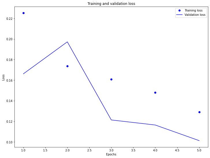
As you can see, the training loss, over time, goes below the validation loss. This means the model has trained well.
Now let’s plot the model training and validation accuracy.
# Plot Training and Validation Accuracy
plt.figure(figsize=(12,9))
plt.plot(epochs, acc, 'bo', label='Training acc')
plt.plot(epochs, val_acc, 'b', label='Validation acc')
plt.title('Training and validation accuracy')
plt.xlabel('Epochs')
plt.ylabel('Accuracy')
plt.legend(loc='lower right')
plt.ylim((0.5,1))
plt.show()
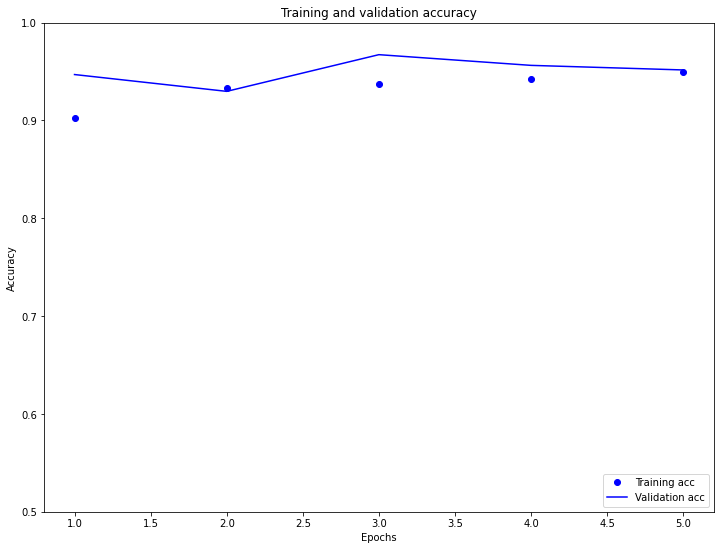
From the above plot, we see that the training and validation accruacy is pretty close. Also, the validation accuracy is more than the training accuracy. This means that the model has trained well and is not overfitting.
Model Evaluation
The above model does not mask the padding applied to the sequences. This can lead to skew if trained on padded sequences and test on un-padded sequences. Ideally we would use masking to avoid this, but as you can see below it only have a small effect on the output.
In case you are unfamiliar with the concept of padding, it’s a technique where we define a constant length for the input text sequence. If the given text length is less than the defined constant length, we pad the sequence with zeros at the end to make the length the same.
If the prediction is >= 0.5, it is positive else it is negative.
# Function to Zero Pad Input Reviews
def pad_to_size(vec, size):
    zeros = [0] * (size - len(vec))
    vec.extend(zeros)
    return vec
# Function to make predictions on Input Reviews
def sample_predict(sample_pred_text, pad):
    encoded_sample_pred_text = encoder.encode(sample_pred_text)

    if pad:
        encoded_sample_pred_text = pad_to_size(encoded_sample_pred_text, 64)
    encoded_sample_pred_text = tf.cast(encoded_sample_pred_text, tf.float32)
    predictions = model.predict(tf.expand_dims(encoded_sample_pred_text, 0))

    return (predictions)
Let’s classify a sample review without applying any text padding.
# Positive Review without Zero Padding
sample_pred_text = ('That restaurant offers great food, must try out.')

predictions = sample_predict(sample_pred_text, pad=False)
print(predictions)
[[0.61917293]]
The model predicts the sentiment for the text as 0.6192 which means it’s a positive review.
Now, let’s try the same review with padding enabled.
# Positive Review with Zero Padding
sample_pred_text = ('That restaurant offers great food, must try out.')

predictions = sample_predict(sample_pred_text, pad=True)
print(predictions)
[[1.2357517]]
Again, the model classifies the text correctly. So, it looks like our model works well with/without padding.
Let’s look at a negative sentiment example.
# Negative Review without Zero Padding
sample_pred_text = ('The food at that restaurant was the worst ever. I would not recommend it to anyone.')

predictions = sample_predict(sample_pred_text, pad=False)
print(predictions)
[[-4.628654]]
The model thinks that this is a negative sentiment which is correct.
# Negative Review with Zero Padding
sample_pred_text = ('The food at that restaurant was the worst ever. I would not recommend it to anyone.')

predictions = sample_predict(sample_pred_text, pad=True)
print(predictions)
[[-6.386962]]
Similaryly, with padding enabled, the model predicts the text sentiment correctly as negative.
Great work on completing this tutorial. You can find the complete source code for this tutorial here.
For more projects and code, follow me on Github.
Please feel free to leave any comments, suggestions, corrections if any, below.
Comments